
Quick answer
For GPA calculation in Excel, list your courses, letter grades and credits in three columns. Look up each grade’s points with XLOOKUP (or VLOOKUP), then divide SUMPRODUCT(credits, points) by SUM(credits). The same formulas work in Google Sheets, and the GPA updates every time you type a new grade.

Key takeaways
- One lookup table turns letters into grade points.
=SUMPRODUCT(C2:C6,D2:D6)/SUM(C2:C6)is the whole GPA formula.- Add a bonus column for a weighted GPA.
- Lock the lookup table with
$signs before copying formulas down.
On this page
A spreadsheet is the easiest way to track your GPA all year. This setup takes five minutes and updates itself every time you type a grade.
Prefer no spreadsheet?Use the GPA calculator instead.Open →Step 1: Lay out the sheet
| Column | A | B | C | D | E |
|---|---|---|---|---|---|
| Header | Course | Grade | Credits | Points | Bonus |
| Row 2 | English 11 | A | 1 | (formula) | 0.5 |
Put a grade table off to the side, for example letters in G2:G14 (A+, A, A−, B+ … F) and points in H2:H14 (4.0, 4.0, 3.7, 3.3 … 0).
Step 2: Look up the grade points
In D2, type:
=XLOOKUP(B2,$G$2:$G$14,$H$2:$H$14)
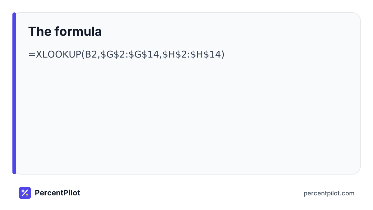
Older Excel? Use =VLOOKUP(B2,$G$2:$H$14,2,FALSE). Copy the formula down the column.
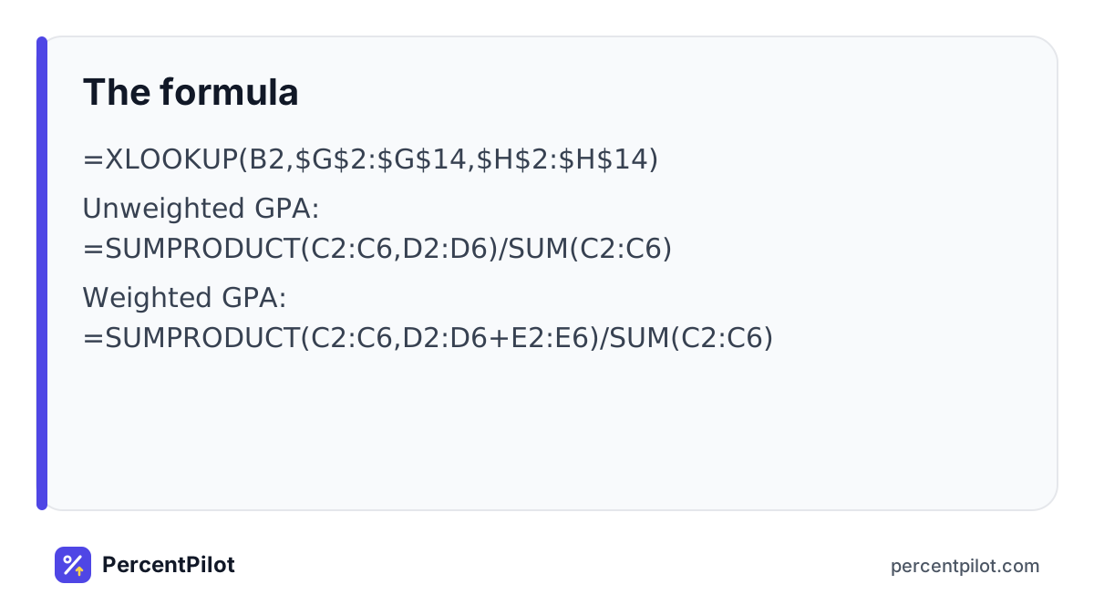
Step 3: The GPA formula
Unweighted GPA: =SUMPRODUCT(C2:C6,D2:D6)/SUM(C2:C6)
Weighted GPA: =SUMPRODUCT(C2:C6,D2:D6+E2:E6)/SUM(C2:C6)
Worked example: Five courses
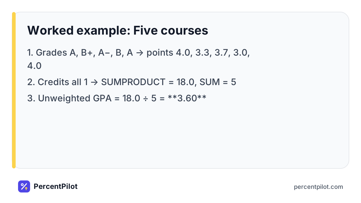
- Grades A, B+, A−, B, A → points 4.0, 3.3, 3.7, 3.0, 4.0
- Credits all 1 → SUMPRODUCT = 18.0, SUM = 5
- Unweighted GPA = 18.0 ÷ 5 = 3.60
Worked example: Weighted column
- Bonus column E: Honors English 0.5, AP U.S. History 1.0, others 0
- SUMPRODUCT of credits × (points + bonus) = 19.5
- Weighted GPA = 19.5 ÷ 5 = 3.90
Tidy-up tips
- Format the GPA cell to two decimals: Home → Number → decrease decimals.
- Add data validation on column B (a dropdown of letters) so a typo can’t break the lookup.
- In Google Sheets,
XLOOKUPandSUMPRODUCTwork the same way.
Accuracy first
If the GPA shows #N/A, a grade in column B doesn’t match the lookup table exactly (for example “A-” typed with a hyphen while the table uses “A−”). Use the same symbol in both places.
What NOT to do
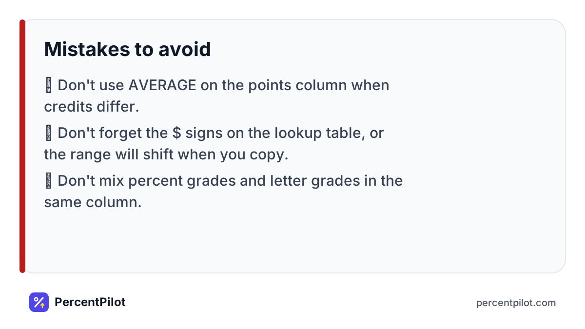
- Don’t use AVERAGE on the points column when credits differ.
- Don’t forget the
$signs on the lookup table, or the range will shift when you copy. - Don’t mix percent grades and letter grades in the same column.
Related: how to calculate GPA by hand, cumulative GPA, all GPA tools.
Where you’ll use this
A spreadsheet is worth setting up if you want to track your GPA across all four years of high school or college. Put each semester on its own tab, then add a summary tab whose cumulative GPA is =SUMPRODUCT of all credits and points divided by the total credits. Every time a grade comes in, the summary updates.
It also helps you test “what if” grades. Add a column called Target, type the grade you hope to earn, and point a second GPA formula at that column. You’ll see your projected GPA next to your current one — useful before finals or when choosing whether to take a class pass/fail. Check your school’s handbook for the scale before you lock in the grade table.
Practice problems (with answers)
Try each one, then check it with the Prefer no spreadsheet?. More tools: all GPA calculators.
- Find the GPA: A (1 cr), B+ (1 cr), A− (1 cr), B (1 cr), A (1 cr). Answer: Quality points: 4.0 × 1 + 3.3 × 1 + 3.7 × 1 + 3.0 × 1 + 4.0 × 1 = 18.00; credits 5 → GPA = 3.60.
- Find the GPA: B (3 cr), A (4 cr), C+ (3 cr). Answer: Quality points: 3.0 × 3 + 4.0 × 4 + 2.3 × 3 = 31.90; credits 10 → GPA = 3.19.
- Find the GPA: A− (1 cr), A− (1 cr), B+ (1 cr), B+ (1 cr). Answer: Quality points: 3.7 × 1 + 3.7 × 1 + 3.3 × 1 + 3.3 × 1 = 14.00; credits 4 → GPA = 3.50.
Frequently asked questions
What is the Excel formula for GPA?
=SUMPRODUCT(credits, grade points)/SUM(credits), for example =SUMPRODUCT(C2:C6,D2:D6)/SUM(C2:C6).
Can I calculate GPA in Google Sheets?
Yes. The same XLOOKUP and SUMPRODUCT formulas work in Google Sheets.
How do I convert percentages to letter grades in Excel?
Use an approximate-match lookup on a table of minimum percentages, such as =XLOOKUP(B2,$J$2:$J$14,$K$2:$K$14,,-1) with the minimums sorted from low to high.
Sources
Spotted an error? Tell us and we will fix it and note the change here.